SOUNotes

DVBI-02 Power BI Desktop & Data Transformation

Data Transformation in Power BI

Data transformation is the process of converting raw data into a clean, structured, and usable format using Power Query Editor.
It helps in improving data quality and preparing data for accurate analysis and reporting.
Users can split columns, merge columns, pivot and unpivot data, filter rows, sort values, and group data.
All transformations are recorded as applied steps, which can be reused automatically during data refresh.

1. Importing Data

The process starts by importing data from sources such as Excel, CSV files, databases, web, or cloud services.
After selecting the data source, users choose the Transform Data option to open Power Query Editor.

2. Data Cleaning

Data cleaning ensures that the dataset is accurate and consistent before analysis.
It includes removing unnecessary rows and columns, handling missing values, removing duplicates, and correcting data types.
Columns can also be renamed for better understanding.

3. Data Transformation (Shaping Data)

Data shaping involves modifying the structure of the data to make it suitable for analysis.
Users can split columns, merge columns, pivot and unpivot data, filter rows, sort values, and group data.
These operations help in organizing data in a meaningful way.

4. Handling Data Issues

Power Query provides methods to handle common data problems.
Missing values can be filled or removed, duplicate records can be eliminated, and outliers can be identified and adjusted.
This improves the reliability of the dataset.

5. Applied Steps

Every transformation performed is recorded as an Applied Step in Power Query Editor.
These steps are saved and automatically applied whenever the data is refreshed.

6. Loading Data

After completing all transformations, users click Close & Apply to load the cleaned data into Power BI.
The transformed data is then ready for modelling and visualization.

Data Transformation Techniques in Power BI

Data transformation is the process of modifying raw data into a structured and analysis-ready format using Power Query Editor.
It involves applying various techniques to clean, shape, and organize data effectively.

1. Filtering Data

Filtering is used to select only relevant rows based on conditions.
Example: Showing only students with marks greater than 50.

2. Sorting Data

Sorting arranges data in ascending or descending order.
Example: Sorting sales data from highest to lowest revenue.

3. Splitting Columns

A single column can be divided into multiple columns based on a delimiter or position.
Example: Splitting “Full Name” into “First Name” and “Last Name”.

4. Merging Columns

Two or more columns can be combined into one column.
Example: Combining “City” and “State” into a single “Location” column.

5. Pivoting Data

Pivoting converts rows into columns for better analysis.
Example: Converting monthly sales data from rows into separate columns for each month.

6. Unpivoting Data

Unpivoting converts columns into rows.
Example: Converting multiple subject columns into a single “Subject” column with marks.

7. Grouping Data (Group By)

Grouping aggregates data based on a category.
Example: Calculating total sales for each region.

8. Replacing Values

Specific values in a dataset can be replaced with new values.
Example: Replacing “N/A” with 0.

9. Changing Data Types

Data types such as text, number, or date can be modified.
Example: Converting a text field into date format for proper analysis.

10. Removing Duplicates

Duplicate records can be removed to maintain data accuracy.
Example: Removing repeated customer entries from a dataset.

Data Cleaning in Power BI

Data cleaning is the process of removing errors and inconsistencies from raw data to improve its quality.
It is performed using Power Query Editor before analysis.
Common cleaning tasks include removing unnecessary rows and columns, handling missing values, removing duplicate records, and correcting data types.
Columns can also be renamed and formatted properly to make data more understandable and consistent.

1. Handling Missing Values

Missing values (null values) can affect calculations and analysis results.
Power BI provides multiple methods to handle them:
- Replace null values with zero, average, or a custom value
- Remove rows or columns containing missing values
- Use Fill Down or Fill Up options to fill values based on nearby data
These techniques help in making the dataset complete and usable.

2. Handling Duplicate Data

Duplicate records can lead to incorrect analysis and misleading results.
Methods to handle duplicates include:
- Using the Remove Duplicates option on selected columns
- Identifying duplicates using grouping and counting techniques
- Keeping only unique records for accurate analysis
Removing duplicates improves data consistency and reliability.

3. Handling Outliers

Outliers are extreme or abnormal values that differ significantly from other data points.
They can distort analysis and affect results.
Methods to handle outliers include:
- Identifying outliers using filters or sorting data
- Removing extreme values that are not relevant
- Replacing outliers with average or median values
- Analyzing outliers separately if they provide useful insights
Proper handling of outliers ensures more accurate and meaningful analysis.

Describe Steps to Remove Duplicates & Outliers.

Removing Duplicates in Power BI

Duplicate records can lead to incorrect analysis and must be removed to ensure data accuracy.

Steps to Remove Duplicates

Open Power BI Desktop and load the dataset
Click on Transform Data to open Power Query Editor
Select the column(s) where duplicates exist
Go to the Home tab and click on Remove Duplicates
Power BI keeps the first occurrence and removes repeated values
Verify the cleaned data and apply changes

Handling Outliers in Power BI

Outliers are extreme or abnormal values that can affect analysis results.

Steps to Handle Outliers

Open Power Query Editor after loading data
Identify outliers by sorting or applying filters on the column
Detect unusually high or low values compared to normal data
Remove outliers by filtering them out or deleting those rows
Alternatively, replace outliers with average or median values
Review the dataset to ensure consistency and accuracy

Data Modelling in Power BI

Data modelling in Power BI is the process of organizing and structuring data by creating relationships between different tables.
It defines how data from multiple sources is connected, allowing users to analyze and visualize data effectively.
Data modelling is mainly performed using Power Pivot, where relationships, calculations, and data structures are created.

Importance of Data modelling in Power BI

1. Improves Performance

Proper data modelling optimizes how data is stored and processed.
It reduces data redundancy and improves the speed of queries and reports.

2. Enables Accurate Calculations

Relationships between tables ensure correct calculations and aggregations.
It helps in generating accurate measures such as totals, averages, and percentages.

3. Simplifies Data Analysis

A well-structured data model makes it easier to understand and analyze data.
Users can easily create reports without dealing with complex data structures.

4. Supports Complex Analysis

Data modelling allows combining data from multiple tables for deeper insights.
It enables advanced analysis using DAX functions and calculations.

5. Better Data Organization

It organizes data into fact and dimension tables, making it more structured and logical.
This improves clarity and usability of data.

6. Enhances Report Design

A good data model simplifies report creation and improves visualization quality.
It allows users to create meaningful dashboards efficiently.

Star Schema

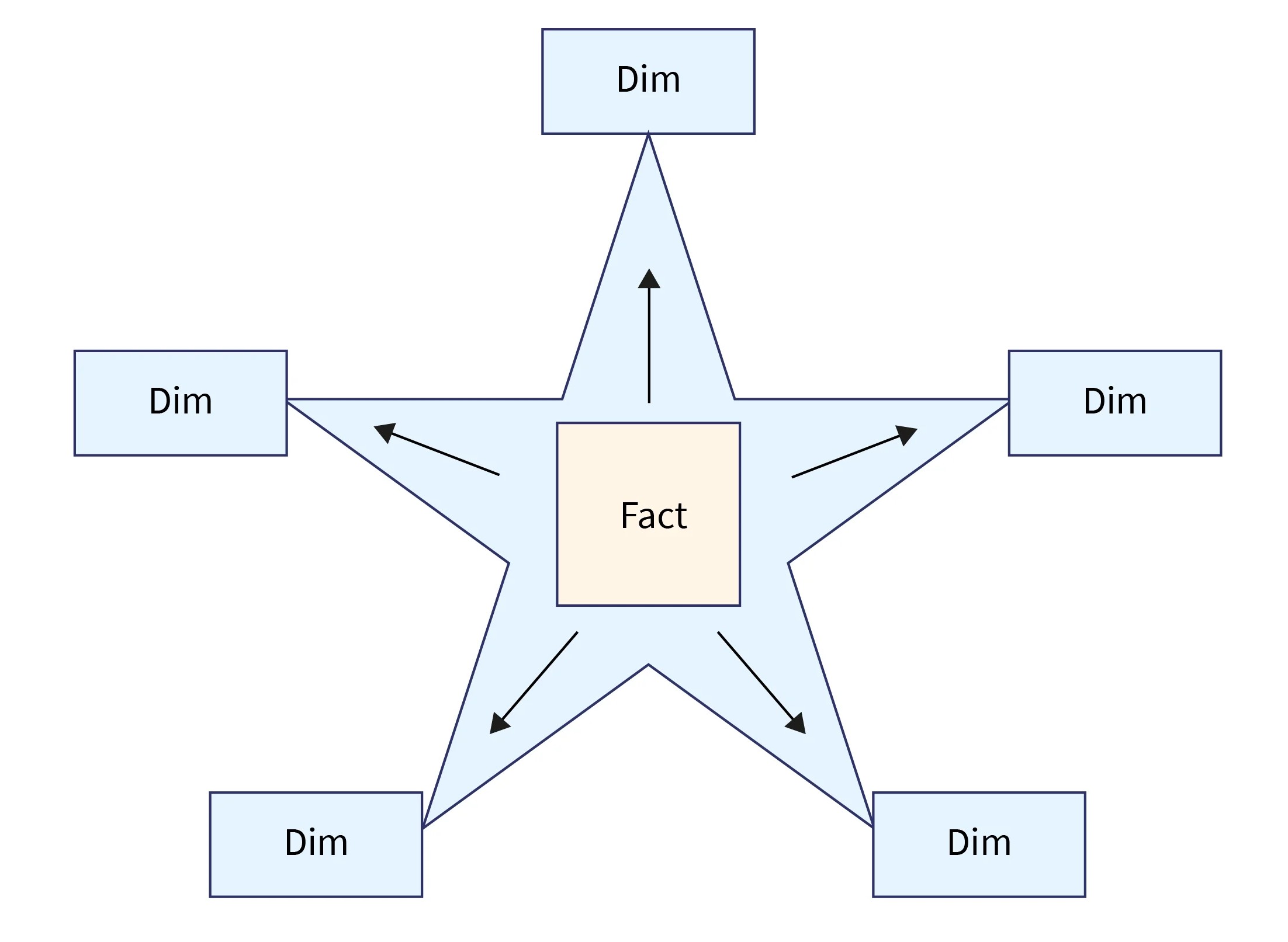
Star schema is a data modelling technique where a central Fact table is connected directly to multiple Dimension tables.
The fact table contains measurable data such as sales, quantity, or revenue, while dimension tables contain descriptive data like product, customer, date, and region.
The structure is simple and widely used in data warehousing and Power BI.

Characteristics of Star Schema

Simple and easy to understand
Fewer joins between tables
Denormalized structure (data may be repeated)
Faster query performance

Advantages

Easy to design and implement
Provides fast data retrieval and analysis
Suitable for reporting and dashboard creation
Recommended for Power BI

Snowflake Schema

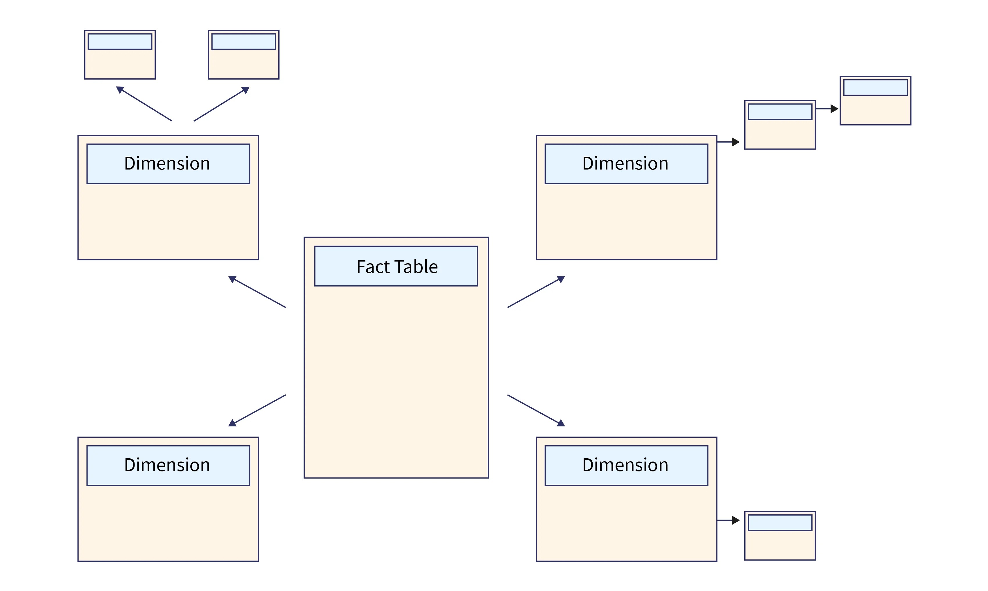
Snowflake schema is a data modelling technique where dimension tables are further divided into multiple related tables.
It follows a normalized structure, reducing data redundancy by splitting data into smaller tables.
This makes the schema more complex compared to star schema.

Characteristics of Snowflake Schema

Complex and normalized structure
More tables and more joins
Reduced data redundancy
Slower query performance

Advantages

Reduces duplication of data
Saves storage space
Improves data consistency and integrity

Disadvantages

Difficult to design and understand
Requires more joins, which can slow down performance
Not preferred for quick analysis in Power BI

Differentiate: Star Schema & Snowflake Schema

Feature	Star Schema	Snowflake Schema
Structure	In Star Schema, a central fact table is directly connected to multiple dimension tables without further division.	In Snowflake Schema, dimension tables are further divided into multiple related sub-tables to reduce redundancy.
Design Type	It follows a denormalized structure where data may be repeated in dimension tables.	It follows a normalized structure where data is organized into multiple smaller tables.
Complexity	The design is simple and easy to understand for users and developers.	The design is complex and requires better understanding of relationships between tables.
Joins	It requires fewer joins between tables, which improves query performance.	It requires more joins due to multiple related tables, which can slow down performance.
Performance	It provides faster data retrieval and is suitable for reporting and analysis.	It provides slower performance compared to star schema due to complex joins.
Data Redundancy	It contains higher data redundancy because data is repeated in dimension tables.	It reduces redundancy by organizing data into separate tables.
Storage	It consumes more storage space because of repeated data.	It saves storage space by minimizing duplication.
Usage in Power BI	It is widely used and recommended in Power BI for better performance and simplicity.	It is less preferred in Power BI because of its complexity and lower performance.

Power BI Desktop Views & Their Functions

Power BI Desktop provides three main views that help users work with data, create reports, and manage relationships effectively.
Each view has a specific purpose in the data analysis and reporting process.

1. Report View

Report View is used to create visualizations and design dashboards.
Users can add charts, tables, graphs, slicers, and other visual elements.
It allows interactive analysis using filters, drill-down, and highlighting features.
This is the main view used for presenting insights.

2. Data View

Data View displays the dataset in tabular format.
Users can inspect data, verify cleaned data, and understand its structure.
It is used to create calculated columns and measures using DAX.
This view helps in checking data accuracy before visualization.

3. Model View

Model View is used to manage relationships between different tables.
It shows a diagram of how tables are connected.
Users can create, edit, or delete relationships and adjust properties like cardinality and filter direction.
It helps in building an efficient data model for analysis.

Data Management in Power BI

Data management in Power BI involves organizing, cleaning, and maintaining data to ensure it is accurate and ready for analysis.
It is mainly performed using Power Query Editor and Data View.

Key Aspects of Data Management

Importing data from multiple sources such as Excel, databases, and cloud services
Cleaning data by removing duplicates, handling missing values, and correcting data types
Transforming data by filtering, sorting, merging, and reshaping datasets
Organizing data into tables for better structure and usability
Ensuring data consistency and quality for reliable analysis

Data Relationship in Power BI

Data relationships in Power BI define how different tables are connected using common fields (keys).
They allow data from multiple tables to be combined and analyzed together in reports and dashboards.
Relationships are created in Model View or using the Manage Relationships option.

Purpose of Data Relationships

To connect tables and enable data interaction
To perform accurate calculations across multiple tables
To support filtering and aggregation in reports

Types of Relationships

1. One-to-One (1 : 1)

Each record in one table is related to exactly one record in another table.
Example: One employee linked to one employee ID record.

2. One-to-Many (1 : * )

One record in a table is related to multiple records in another table.
Example: One customer can have multiple orders.
This is the most commonly used relationship.

3. Many-to-Many ( _ : _ )

Multiple records in one table are related to multiple records in another table.
Example: Students and courses (a student can take many courses, and a course can have many students).

Key Properties of Relationships

1. Cardinality

Defines the type of relationship between tables (1:1, 1:_, _:*).

2. Cross Filter Direction

Determines how filters are applied between related tables (single or both directions).

3. Active and Inactive Relationships

Active relationships are used by default in analysis.
Inactive relationships can be activated when needed using DAX functions.

Importance of Data Relationships

Enables combining data from multiple tables
Ensures accurate analysis and reporting
Improves data model efficiency
Helps create meaningful visualizations

Relationship Creation in Power BI

Relationship creation is the process of connecting different tables based on common fields (keys).
It allows data from multiple tables to be used together in analysis and reporting.

Steps to Create Relationships

Go to Model View in Power BI Desktop
Identify common columns (such as ID, Customer ID, Product ID)
Drag and drop one column onto another to create a relationship
Alternatively, use the Manage Relationships option

Types of Relationships

One-to-One ( 1 : 1 ): Each record in one table is related to one record in another table
One-to-Many ( 1 : * ): One record in a table is related to multiple records in another table
Many-to-Many ( _ : _ ): Multiple records in both tables are related to each other

Relationship Properties

Cardinality: Defines the type of relationship (1:1, 1:_ , _ : * )
Cross Filter Direction: Controls how filters are applied between tables
Active/Inactive Relationship: Determines whether the relationship is currently used in analysis
Proper relationship creation ensures accurate calculations, better data analysis, and efficient report generation.

The Process of Data Modelling in Power BI

Data modelling is the process of organizing data and creating relationships between tables to enable effective analysis.
It is performed after data is cleaned and transformed.

1. Loading Data

After cleaning and transformation, data is loaded into Power BI using Close & Apply.
The data becomes available in Data View and Model View.

2. Creating Relationships

Tables are connected using common fields such as IDs or keys.
Relationships are created in Model View by dragging one column to another.

3. Defining Relationship Types

Relationships are defined as one-to-one, one-to-many, or many-to-many based on data structure.
Proper relationship type ensures accurate data linking.

4. Setting Relationship Properties

Properties such as cardinality and cross-filter direction are configured.
Active and inactive relationships are managed for correct analysis.

5. Organizing Data Model

Tables are structured into fact and dimension tables.
A proper schema (like star schema) is used for better performance.

6. Creating Calculations

Measures and calculated columns are created using DAX.
These calculations help in advanced analysis and reporting.