MLDNN-02 Supervised & Unsupervised Learning

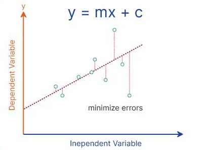
Linear Regression

• Linear Regression is a supervised learning algorithm used to predict continuous numerical values.
• It shows the relationship between an input variable and an output variable using a straight line.
• It is one of the simplest and most commonly used algorithms in Machine Learning.

Mathematical Representation

• Linear Regression is represented by the equation:
  • y = mx + c
• Where:
  • y = predicted output
  • x = input feature
  • m = slope (rate of change)
  • c = intercept (value of y when x = 0)

How Linear Regression Works

• Data points are plotted on a graph.
• A straight line (best fit line) is drawn through the data.
• The line is chosen such that it minimizes the prediction error.
• This is usually done using the Least Squares Method.

Derivation

• A straight line is assumed between input and output.
• The slope (m) represents how much y changes when x changes.
• The intercept (c) represents the starting point of the line.
• The best values of m and c are calculated such that the error between predicted and actual values is minimum.
• Thus, the model fits a line that best represents the data.

Use in Prediction Problems

• Linear Regression is used when we need to predict continuous values based on input data.
• It finds a relationship between variables and uses it to make predictions for new data.

Example

• Predicting student marks based on study hours:
  • If study hours increase, marks also increase.
  • The model learns this pattern and predicts marks for new students.
• Predicting salary based on experience:
  • More experience generally leads to higher salary.
  • The model uses past data to estimate future salary.

Applications

• House price prediction
• Sales forecasting
• Salary prediction
• Temperature prediction

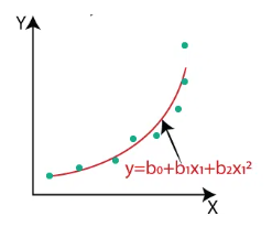
Polynomial Regression

• Polynomial Regression is a type of regression algorithm used to model non-linear relationships between input and output variables.
• It is an extension of Linear Regression but fits a curved line instead of a straight line.
• It is used when the data shows a non-linear pattern.

Mathematical Representation

• The equation of Polynomial Regression is:
  y = b₀ + b₁x + b₂x² + b₃x³ + ... + bₙxⁿ

• Where:

  • y = predicted output
  • x = input variable
  • b₀, b₁, b₂, … = coefficients
  • n = degree of the polynomial

How Polynomial Regression Works

• The model transforms the original input variable into higher-degree terms (x², x³, etc.).
• These new features allow the model to fit a curved relationship in the data.
• It then applies linear regression on these transformed features.
• The goal is to minimize the error between predicted and actual values.

Example

• Suppose we have data for study hours and marks:
  • At first, marks increase slowly, then rapidly.
• A straight line cannot fit this pattern properly.
• Polynomial Regression fits a curve that better represents the data.

Advantages

• Can model complex and non-linear relationships.
• Provides better accuracy than linear regression for curved data.
• Flexible due to adjustable polynomial degree.

Disadvantages

• Can lead to overfitting if the degree is too high.
• More complex than linear regression.
• Requires careful selection of polynomial degree.

Applications

• Predicting growth trends
• Sales forecasting with seasonal variation
• Temperature and weather prediction
• Biological and scientific data modeling

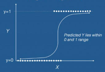
Logistic Regression

• Logistic Regression is a supervised learning algorithm used for classification problems.
• It predicts the probability of an output belonging to a particular category.
• Unlike Linear Regression, it is used when the output is categorical (e.g., Yes/No, 0/1).

How Logistic Regression Works

• Logistic Regression uses a mathematical function called the sigmoid function.
• The sigmoid function converts any value into a range between 0 and 1.
• Based on this probability, the model classifies the output into a specific category.
• For example, if the probability is greater than 0.5, it may classify as “Yes”, otherwise “No”.

Key Features

• It is mainly used for binary classification problems.
• It can also be extended to multiclass classification.
• It provides probability-based outputs, making it easy to interpret.

Applications of Logistic Regression

• Spam Detection: Classifies emails as spam or not spam based on content and keywords.
• Medical Diagnosis: Predicts whether a patient has a disease or not based on symptoms and test results.
• Credit Card Fraud Detection: Identifies whether a transaction is fraudulent or genuine.
• Student Result Prediction: Predicts whether a student will pass or fail based on study data.
• Customer Churn Prediction: Predicts whether a customer will continue a service or leave.

K-Nearest Neighbors (KNN)

• K-Nearest Neighbors (KNN) is a supervised learning algorithm used for both classification and regression problems.
• It works based on the idea that similar data points are located close to each other.
• It classifies new data points by comparing them with the nearest existing data points.

How KNN Works

• Choose the number of neighbors (K value).
• Calculate the distance between the new data point and all existing data points.
• Select the K nearest neighbors based on distance.
• For classification, assign the class that is most common among the neighbors.
• For regression, take the average of the nearest values.

Example

• Suppose we have two categories: Apple and Orange.
• Each fruit is described using features like color, size, and shape.
• When a new fruit is given, the algorithm checks its nearest neighbors.
• If most of the nearest neighbors are Apples, it classifies the new fruit as Apple.
• If most neighbors are Oranges, it classifies it as Orange.

Effect of K on Performance

• Small K (e.g., K = 1)

  • Model becomes sensitive to noise.
  • Can lead to overfitting (very specific to training data).

• Large K (e.g., K = 10 or more)

  • Model becomes more generalized.
  • Can lead to underfitting (loses important details).

• Optimal K

  • A moderate value (like 3, 5, or 7) is usually chosen.
  • It balances accuracy and generalization.

Key Points

• KNN is a simple and easy-to-understand algorithm.
• It does not require a training phase (lazy learning).
• The choice of K value is very important for accuracy.

Applications

• Recommendation systems
• Image recognition
• Medical diagnosis
• Customer segmentation

Support Vector Machine (SVM)

• Support Vector Machine (SVM) is a supervised learning algorithm used for classification and regression problems.
• It works by finding the best boundary (called a hyperplane) that separates data into different classes.
• The main objective of SVM is to maximize the distance between the boundary and the nearest data points.

How SVM Works

• Data points are plotted in a feature space.
• SVM finds an optimal hyperplane that separates different classes.
• The data points closest to the boundary are called support vectors.
• These support vectors play a key role in defining the decision boundary.

Concept of Hyperplane

• A hyperplane is a decision boundary that separates data points into different classes.
• In 2D, it is a straight line; in 3D, it becomes a plane.
• SVM finds the optimal hyperplane that best divides the data into classes.

Concept of Margin

• Margin is the distance between the hyperplane and the nearest data points (support vectors).
• SVM tries to maximize this margin to improve model accuracy and generalization.
• A larger margin leads to better separation between classes and reduces classification errors.

Concept of Kernel

• Kernel is a function used to transform data into a higher-dimensional space.
• It is useful when data is not linearly separable.
• By using kernels, SVM can create complex boundaries to separate data.

Common Types of Kernels

• Linear Kernel: Used when data is linearly separable.
• Polynomial Kernel: Used for curved relationships.
• RBF (Radial Basis Function): Used for complex, non-linear data.

Example

• Suppose we want to classify students as Pass or Fail based on marks.
• SVM finds a boundary that separates pass and fail students clearly.
• If the data is not linearly separable, a kernel is used to create a better boundary.

Accuracy

• Accuracy measures how many predictions made by the model are correct out of the total predictions.
• It gives an overall idea of the model’s performance.
• Example: If 90 out of 100 predictions are correct, accuracy is 90%.

Precision

• Precision measures how many of the predicted positive cases are actually correct.
• It focuses on the correctness of positive predictions.
• Example: Out of all emails predicted as spam, how many are truly spam.

Recall

• Recall measures how many actual positive cases are correctly identified by the model.
• It focuses on capturing all real positive instances.
• Example: Out of all actual spam emails, how many were correctly detected.

F1-Score

• F1-score is the harmonic mean of precision and recall.
• It provides a balance between precision and recall, especially when there is an imbalance in data.
• It is useful when both false positives and false negatives are important.

Why These Metrics Are Important

• They help evaluate how well a machine learning model performs.
• Accuracy alone may be misleading when data is imbalanced.
• Precision is important when false positives are costly (e.g., spam detection).
• Recall is important when missing a positive case is dangerous (e.g., medical diagnosis).
• F1-score provides a balanced measure when both precision and recall matter.

Define Accuracy, Precision, Recall and F1-Score using a confusion matrix.

Confusion Matrix

• A confusion matrix is a table used to evaluate the performance of a classification model.
• It compares actual values with predicted values.

	Predicted Positive	Predicted Negative
Actual Positive	True Positive (TP)	False Negative (FN)
Actual Negative	False Positive (FP)	True Negative (TN)

Accuracy

• Accuracy measures the overall correctness of the model.
• Formula: (TP + TN) / (TP + TN + FP + FN)
• It shows how many predictions are correct out of total predictions.

Precision

• Precision measures how many predicted positive cases are actually correct.
• Formula: TP / (TP + FP)
• It focuses on reducing false positives.

Recall

• Recall measures how many actual positive cases are correctly identified.
• Formula: TP / (TP + FN)
• It focuses on reducing false negatives.

F1-Score

• F1-score is the harmonic mean of precision and recall.
• Formula: 2 × (Precision × Recall) / (Precision + Recall)
• It balances both precision and recall.

When is Accuracy not a good evaluation metric? Explain using an imbalanced dataset example.

When Accuracy is Not Suitable

• Accuracy is not a reliable metric when the dataset is imbalanced, meaning one class has significantly more data than the other.
• In such cases, the model may appear to perform well by predicting only the majority class, while ignoring the minority class.
• This leads to misleading results, as the model does not truly learn meaningful patterns.

Imbalanced Dataset Example

• Suppose we have a dataset of 100 emails:

  • 95 are Not Spam
  • 5 are Spam

• If a model predicts all emails as “Not Spam”:

  • Correct predictions = 95
  • Wrong predictions = 5
  • Accuracy = 95%

• Even though accuracy is high, the model fails to identify any spam emails.

• This means the model is useless for detecting spam, despite showing good accuracy.

Why This is a Problem

• The model ignores the minority class (Spam), which is often the most important.
• In real-world applications like fraud detection or medical diagnosis, missing positive cases can be dangerous.
• Therefore, relying only on accuracy can lead to incorrect conclusions about model performance.

Better Alternatives

• Precision: Focuses on correctness of positive predictions.
• Recall: Focuses on detecting all actual positive cases.
• F1-score: Balances both precision and recall.

Explain ROC Curve and ROC-AUC

ROC Curve (Receiver Operating Characteristic Curve)

• ROC Curve is a graphical tool used to evaluate the performance of classification models.
• It shows the trade-off between True Positive Rate (TPR) and False Positive Rate (FPR) at different threshold values.
• Each point on the curve represents a different decision threshold.

Key Terms

• True Positive Rate (TPR) = TP / (TP + FN)

  • Also known as Recall, it measures how many actual positives are correctly identified.

• False Positive Rate (FPR) = FP / (FP + TN)

  • It measures how many negative cases are incorrectly classified as positive.

ROC-AUC (Area Under the Curve)

• ROC-AUC represents the area under the ROC curve.

• It provides a single value to summarize the model’s performance across all thresholds.

• Interpretation of AUC values:

  • 1.0 → Perfect model
  • 0.9 → Excellent model
  • 0.7–0.8 → Good model
  • 0.5 → Random guessing

Why ROC-AUC is Useful

• It evaluates model performance across all classification thresholds, not just one.
• It provides a balanced view of performance between true positives and false positives.
• It is less affected by class imbalance compared to accuracy.
• It allows easy comparison between multiple models—higher AUC indicates better performance.

Example

• If Model A has AUC = 0.90 and Model B has AUC = 0.75, Model A is considered better at distinguishing between classes.

Describe K-Means Clustering algorithm with step-by-step procedure.

What is K-Means Clustering

• K-Means Clustering is an unsupervised learning algorithm used to group similar data points into clusters.
• It divides the dataset into K number of clusters based on similarity.
• Each cluster has a center point called a centroid.

Step-by-Step Procedure

1. Choose number of clusters (K)

• Decide how many clusters you want to form in the dataset.

2. Initialize centroids

• Randomly select K points as initial centroids.

3. Assign data points

• Calculate the distance of each data point from all centroids.
• Assign each point to the nearest centroid.

4. Update centroids

• Recalculate the centroid of each cluster by taking the average of all points in that cluster.

5. Repeat the process

• Repeat steps 3 and 4 until the centroids no longer change or stabilize.

6. Final clusters

• The final groups formed are the clusters with similar data points.

Example

• Grouping customers based on income and spending habits into different categories.

Compare Hierarchical Clustering and DBSCAN. Mention advantages and limitations.

Hierarchical Clustering

• Hierarchical Clustering builds clusters in a tree-like structure called a dendrogram.
• It can be either agglomerative (bottom-up) or divisive (top-down).
• It does not require specifying the number of clusters in advance.

DBSCAN (Density-Based Spatial Clustering of Applications with Noise)

• DBSCAN is a density-based clustering algorithm.
• It groups data points based on density and identifies outliers as noise.
• It requires parameters like minimum points and distance (epsilon).

Key Differences

Aspect	Hierarchical Clustering	DBSCAN
Approach	Builds clusters step-by-step in a hierarchy	Groups data based on density of points
Cluster Shape	Works well for simple structures	Detects clusters of arbitrary shapes
Handling Noise	Does not handle noise effectively	Identifies and removes noise/outliers
Number of Clusters	No need to predefine K	No fixed number, depends on density

Advantages

Hierarchical Clustering

• Easy to understand and visualize (dendrogram).
• No need to specify number of clusters initially.

DBSCAN

• Can find clusters of any shape.
• Effectively handles noise and outliers.
• Works well with large datasets.

Limitations

Hierarchical Clustering

• Computationally expensive for large datasets.
• Sensitive to noise and outliers.

DBSCAN

• Choosing parameters (epsilon and min points) is difficult.
• Not suitable when data has varying densities.

Principal Component Analysis (PCA)

• PCA is an unsupervised learning technique used for dimensionality reduction.
• It transforms a large number of features into a smaller set of new variables called principal components.
• These components capture the most important information (maximum variance) in the data.

How PCA Works

• The data is first standardized so that all features are on the same scale.
• PCA computes the directions (principal components) where the data varies the most.
• The first principal component captures the highest variance, the second captures the next highest, and so on.
• These components are orthogonal (independent) to each other.

How PCA Reduces Dimensionality

• Instead of using all original features, PCA selects only the top few principal components.
• These components retain most of the important information from the dataset.
• Less important features (with low variance) are removed.
• This reduces the number of dimensions while preserving the overall structure of the data.

Example

• A dataset with 10 features can be reduced to 2 or 3 principal components while still retaining most of the information.
• This makes computation faster and visualization easier.

Advantages

• Reduces complexity of the dataset.
• Improves model performance and speed.
• Removes redundant and correlated features.

Differentiate between PCA and LDA

Principal Component Analysis (PCA)

• PCA is an unsupervised technique used for dimensionality reduction.
• It focuses on maximizing variance in the data.
• It does not consider class labels.
• It is mainly used for data compression and visualization.

Linear Discriminant Analysis (LDA)

• LDA is a supervised technique used for dimensionality reduction and classification.
• It focuses on maximizing the separation between different classes.
• It uses class labels to improve class discrimination.
• It is mainly used when classification is required.

Key Differences

Aspect	PCA (Principal Component Analysis)	LDA (Linear Discriminant Analysis)
Learning Type	Unsupervised	Supervised
Objective	Maximize variance	Maximize class separation
Use of Labels	Does not use labels	Uses class labels
Application	Data reduction, visualization	Classification, feature reduction

When to Prefer LDA over PCA

• When the dataset has labeled data and the goal is classification.
• When we want to maximize separation between different classes.
• When improving classification accuracy is more important than just reducing dimensions.

---