MLDNN-03 Introduction to Deep Learning

Deep Learning (DL)

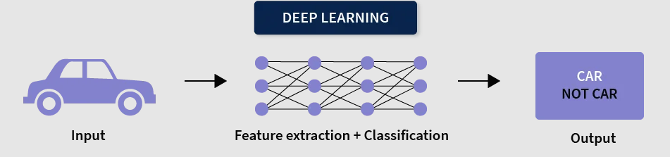
• Deep Learning is a subset of Machine Learning that uses artificial neural networks with multiple layers to learn from data.
• It is inspired by the structure of the human brain and is capable of learning complex patterns automatically.
• It works especially well with large datasets and complex problems.

How Deep Learning Works

• Deep learning models consist of multiple layers: input layer, hidden layers, and output layer.
• The input layer receives raw data such as images, text, or audio.
• Hidden layers process the data and extract important features step by step.
• The output layer gives the final prediction or result.
• Each layer learns more complex patterns than the previous one.

Key Features of Deep Learning

• Uses multi-layer neural networks (deep neural networks).
• Automatically extracts features from raw data.
• Handles large and complex datasets efficiently.
• Provides high accuracy for tasks like image and speech recognition.

Applications of Deep Learning in Real-World Domains

1. Healthcare

• Deep Learning is widely used in medical diagnosis and treatment planning.
• It helps in analyzing medical images such as X-rays, MRIs, and CT scans to detect diseases.
• It can identify patterns that are difficult for humans to detect.
• Example: Detecting tumors, predicting diseases like cancer, and assisting doctors in diagnosis.

2. Finance

• Deep Learning is used in the finance sector for fraud detection and risk analysis.
• It analyzes large amounts of transaction data to identify unusual patterns.
• It helps in making better investment decisions and predicting market trends.
• Example: Detecting fraudulent credit card transactions and predicting stock price movements.

3. Computer Vision

• Computer Vision is a field where machines interpret and understand visual data like images and videos.
• Deep Learning helps in recognizing objects, faces, and scenes accurately.
• It is used in security systems, automation, and image processing.
• Example: Face recognition systems, self-driving cars, and object detection in images.

4. Natural Language Processing (NLP)

• Deep Learning helps machines understand and process human language.
• It is used in translation, chatbots, and text analysis.
• Example: Language translation apps and virtual assistants.

5. Speech Recognition

• Deep Learning converts speech into text and understands voice commands.
• Example: Voice assistants like Siri and Google Assistant.

Artificial Neural Network (ANN)

• An Artificial Neural Network (ANN) is a computational model inspired by the human brain.
• It consists of interconnected nodes (neurons) that process information.
• ANN is used to recognize patterns, learn from data, and make predictions.

Basic Structure of ANN

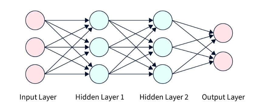
1. Input Layer

• This layer receives the input data from the outside world.
• Each neuron represents a feature of the data.

2. Hidden Layer(s)

• These layers process the input data.
• They perform calculations and extract important patterns.
• There can be one or multiple hidden layers in a network.

3. Output Layer

• This layer produces the final result or prediction.
• It gives the output in the required format (e.g., class label or value).

Working of ANN

• Input data is passed to the input layer.
• Each neuron multiplies the input by a weight and adds a bias.
• The result is passed through an activation function.
• The processed data moves through hidden layers.
• Finally, the output layer produces the result.
• The network learns by adjusting weights and biases to reduce error.

Example

• In image recognition, the input layer receives pixel values.
• Hidden layers detect features like edges and shapes.
• The output layer identifies the object (e.g., cat or dog).

Components of a Neuron in an ANN

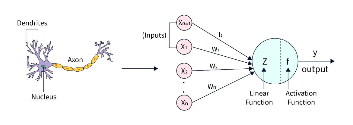
1. Inputs (x₁, x₂, …, xₙ)

• These are the input values or features provided to the neuron.
• They represent the data that the model receives.

2. Weights (w₁, w₂, …, wₙ)

• Each input is multiplied by a weight that represents its importance.
• Higher weight means greater influence on the output.

3. Bias (b)

• Bias is an additional value added to the weighted sum.
• It helps in shifting the output and improving model performance.

4. Weighted Sum (z)

• It is the sum of all inputs multiplied by their weights plus bias: z = w₁x₁ + w₂x₂ + ... + wₙxₙ + b

5. Activation Function

• It decides whether the neuron should be activated or not.
• It converts the weighted sum into the final output.

6. Output (y)

• The final result produced by the neuron after applying the activation function.

Perceptron Model

• The Perceptron is the simplest form of an Artificial Neural Network.
• It is a single-layer neural network used for binary classification (Yes/No, 0/1).
• It takes input values, processes them, and produces an output based on a decision rule.

Structure of Perceptron

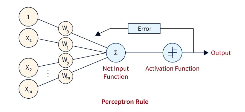
• It consists of input values, weights, bias, and an activation function.
• Each input is assigned a weight that represents its importance.
• A bias is added to adjust the final output.
• The activation function decides the final result.

Mathematical Representation

The perceptron calculates a weighted sum of inputs:

• z = w1x1 + w2x2 + w3x3 + ... + b The output is then passed through an activation function:
• y = f(z) For a simple step function:
  • If z ≥ 0 → Output = 1
  • If z < 0 → Output = 0

Explanation of Terms

• x₁, x₂, …, xₙ (Inputs): These are the input features given to the model.
• w₁, w₂, …, wₙ (Weights): These represent the importance of each input.
• b (Bias): A constant value added to shift the decision boundary.
• z (Weighted Sum): The combined value of inputs and weights plus bias.
• f(z) (Activation Function): Determines the final output based on z.
• y (Output): The final prediction (0 or 1).

Working of Perceptron

• Input values are multiplied by their respective weights.
• All values are added together along with bias.
• The result (z) is passed to the activation function.
• The activation function produces the final output (0 or 1).
• The model learns by adjusting weights when predictions are incorrect.

Example

• Predict whether a student will pass or fail:
  • Inputs: study hours, attendance
  • Output: Pass (1) or Fail (0)
• The perceptron combines inputs and makes a decision based on a threshold.

Activation Functions

• An activation function is a mathematical function used in neural networks to decide whether a neuron should be activated or not.
• It takes the weighted sum of inputs (including bias) and converts it into an output signal.
• It controls how much information should pass to the next layer in the network.
• Activation functions help the network learn and represent complex patterns in data.

Why it is Important

• It introduces non-linearity, which allows neural networks to learn complex and real-world relationships.
• Without activation functions, the network would behave like a simple linear model and cannot solve complex problems.
• It helps neurons decide whether to activate based on input values.
• It improves the learning ability and accuracy of the model.
• It enables deep neural networks to learn multiple levels of abstraction (from simple to complex features).
• It allows the network to handle tasks like image recognition, speech processing, and classification effectively.

Example

• In image recognition, activation functions help detect edges, shapes, and objects step by step.
• Without activation functions, the network would not be able to distinguish between complex patterns in images.

1. Sigmoid Function

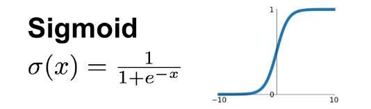
• The sigmoid function gives output values between 0 and 1.
• It is mainly used for binary classification problems.
• Formula: f(x) = 1 / (1 + e⁻ˣ)
• Example: Predicting whether an email is spam or not.

2. Tanh Function

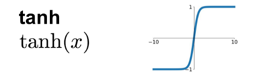
• The tanh function gives output values between -1 and +1.
• It is zero-centered, which helps in better learning compared to sigmoid.
• Example: Sentiment analysis (positive, negative, neutral).

3. ReLU (Rectified Linear Unit)

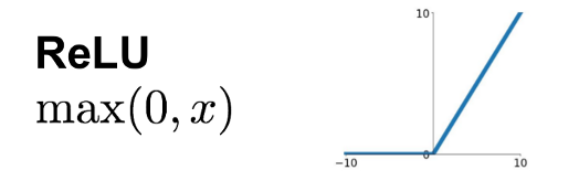
• ReLU outputs 0 if the input is negative, otherwise it returns the input value.
• It is simple, fast, and widely used in deep learning models.
• Formula: f(x) = max(0, x)
• Example: Used in hidden layers of neural networks.

4. Softmax Function

• Softmax converts values into probabilities that sum to 1.
• It is used in multi-class classification problems.
• Example: Classifying an image as cat, dog, or bird.

Softmax Activation Function & its Role in Multi-Class Classification

• Softmax is an activation function used in neural networks for multi-class classification problems.
• It converts raw output values (logits) into probabilities.
• The output values are in the range of 0 to 1, and their total sum is always equal to 1.

How Softmax Works

• It takes multiple input values and applies an exponential function to each.
• Then, each value is divided by the sum of all exponential values.
• This produces a probability distribution over all classes.

Role in Multi-Class Classification

• Softmax helps the model decide which class is most likely among multiple options.
• Each output neuron represents one class.
• The class with the highest probability is selected as the final prediction.

Example

• Suppose a model classifies an image as:
  • Cat → 0.7
  • Dog → 0.2
  • Rabbit → 0.1
• The model predicts "Cat" because it has the highest probability.

Optimization in Deep Learning

• Optimization is the process of improving a deep learning model by reducing its error (loss).
• It involves adjusting the model’s weights and biases to make better predictions.

Why Optimization is Necessary

• Initially, the model makes incorrect predictions due to random weights.
• Optimization helps the model learn from errors and improve accuracy step by step.
• It minimizes the loss function, which measures the difference between predicted and actual values.
• Without optimization, the model cannot learn or improve its performance.

How it Works

• The model makes predictions and calculates the loss.
• An optimization algorithm (like gradient descent) updates the weights.
• This process is repeated until the loss is minimized.

Example

• It is like improving your exam score by correcting mistakes after each test.
• With each correction, your performance becomes better.

Gradient Descent

• Gradient Descent is an optimization algorithm used in Machine Learning and Deep Learning to minimize the error (loss) of a model.
• It works by adjusting the model’s weights step by step so that the predictions become closer to the actual values.
• The main goal is to find the best values of parameters that give minimum loss.

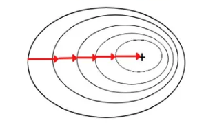
Basic Idea

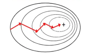
• Imagine the error as a curve (loss function).
• Gradient Descent tries to find the lowest point on this curve.
• It moves step by step in the direction where the error decreases the most.

How Gradient Descent Works

1. Initialize Parameters

• The model starts with random values of weights.

2. Calculate Loss

• The model makes predictions and compares them with actual values.
• The difference between them is called loss or error.

3. Compute Gradient

• The gradient tells how much and in which direction the weights should change to reduce error.

4. Update Weights

• Weights are updated in the opposite direction of the gradient.
• This step is controlled by a parameter called learning rate.

5. Repeat Process

• Steps are repeated until the loss becomes very small or stops decreasing.

Simple Example

• Imagine you are trying to reach the bottom of a hill in the dark.
• You cannot see the whole path, so you take small steps downward.
• At each step, you check the slope and move in the direction where the ground goes down.
• Eventually, you reach the lowest point.
• Similarly, Gradient Descent adjusts weights step by step to reach minimum error.

Key Points

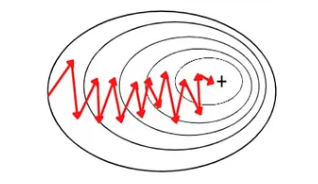
• Learning rate controls how big each step is.
• Too large learning rate may skip the minimum point.
• Too small learning rate makes learning slow.

Differences between AI, ML, and DL

Aspect	AI (Artificial Intelligence)	ML (Machine Learning)	DL (Deep Learning)
Nature of Technology	General concept of creating intelligent systems	Technique enabling machines to learn from data	Advanced technique based on neural networks
Working Style	Uses rules, logic, and learning methods	Uses statistical algorithms to learn patterns	Uses layered neural networks to learn automatically
Feature Handling	May rely on predefined rules	Requires manual feature selection	Automatically extracts features from raw data
Data Type Handling	Works with simple or structured data	Mainly works with structured data	Handles complex unstructured data (images, audio, text)
Performance Level	Moderate, depends on system design	Good with proper data	High for complex, large-scale problems

DL in Image Recognition

• Deep Learning uses neural networks, especially Convolutional Neural Networks (CNNs), to analyze and understand images.
• The model processes images through multiple layers to extract features step by step.
• In the initial layers, simple features like edges, lines, and colors are detected.
• In deeper layers, complex patterns such as shapes, textures, and objects are identified.
• The final layer classifies the image into categories based on learned patterns.
• This approach allows the system to automatically learn features without manual programming.
• Example: Face recognition in smartphones, object detection in images, and handwriting recognition.

DL in Natural Language Processing (NLP)

• Deep Learning is used to process and understand human language in both text and speech form.
• It uses models like Recurrent Neural Networks (RNNs) and Transformers to capture context and meaning.
• The system learns patterns in language such as grammar, sentence structure, and word relationships.
• It can perform tasks like translation, text generation, sentiment analysis, and question answering.
• Deep Learning enables machines to understand context rather than just individual words.
• Example: Language translation (English to Hindi), chatbots, virtual assistants, and text summarization.

Differentiate between Batch Gradient Descent, Stochastic Gradient Descent, and Mini-Batch Gradient Descent.

Batch Gradient Descent

• Batch Gradient Descent uses the entire dataset to compute the gradient in each iteration.
• It calculates the average error over all training examples before updating weights.

Advantages

• Provides stable and accurate updates.
• Converges smoothly towards the minimum.

Disadvantages

• Slow for large datasets.
• Requires high memory and computation power.

Stochastic Gradient Descent (SGD)

• Stochastic Gradient Descent updates weights using one data point at a time.
• It performs frequent updates after each training example.

Advantages

• Faster and requires less memory.
• Can escape local minima due to random updates.

Disadvantages

• Updates are noisy and less stable.
• May not converge smoothly to the exact minimum.

Mini-Batch Gradient Descent

• Mini-Batch Gradient Descent uses a small subset (batch) of data to update weights.
• It is a combination of Batch and Stochastic Gradient Descent.

Advantages

• Faster than batch and more stable than SGD.
• Efficient for large datasets and widely used in practice.

Disadvantages

• Requires choosing appropriate batch size.
• Performance depends on batch size selection.

Aspect	Batch Gradient Descent	Stochastic Gradient Descent (SGD)	Mini-Batch Gradient Descent
Approach	Uses entire dataset per update	Uses one data point per update	Uses small subset (batch) per update
Gradient Calculation	Average error over all training examples	Error from single example	Average error over batch
Speed	Slow	Fast	Moderate and efficient
Memory Usage	High	Low	Moderate
Stability	High (smooth convergence)	Low (noisy updates)	Balanced stability
Convergence	Smooth, accurate	Fluctuates, less precise	Faster and relatively stable
Handling Large Data	Not suitable	Suitable	Highly suitable
Advantages	Stable, accurate updates	Fast, low memory, escapes local minima	Balanced speed and stability, widely used
Disadvantages	Slow, computationally expensive	Noisy, unstable convergence	Depends on batch size selection
Data per Update	Entire dataset	One data point	Small batch
Typical Usage	Small datasets	Online learning	Deep learning (most common)

A neuron receives inputs 0.5 and 0.8 with weights 0.4 and 0.6 respectively. Calculate the output using Sigmoid activation (assume bias = 0).

Step 1: Calculate Weighted Sum (z)

• Formula: z = (w₁x₁ + w₂x₂ + b)

• Given:

  • x₁ = 0.5, w₁ = 0.4
  • x₂ = 0.8, w₂ = 0.6
  • b = 0

• Calculation:

  • z = (0.4 × 0.5) + (0.6 × 0.8) + 0
  • z = 0.2 + 0.48
  • z = 0.68

Step 2: Apply Sigmoid Function

• Formula: σ(z) = 1 / (1 + e⁻ᶻ)
• Substitute z = 0.68: σ(0.68) = 1 / (1 + e⁻⁰·⁶
• Approximate value: e⁻⁰·⁶⁸ ≈ 0.506
• Final calculation:
  • σ(0.68) = 1 / (1 + 0.506)
  • σ(0.68) ≈ 1 / 1.506
  • σ(0.68) ≈ 0.664

Final Output: The output of the neuron using Sigmoid activation is approximately 0.66.

---